
Pythagorean W% v. Same Year W%

A few years ago I published an article on estimating a team’s W% in the subsequent season using either their actual W%, Expected W% (EW%, Pythagenpat using R/RA), or Predicted W% (PW%, Pythagenpat using Runs Created/Runs Created Allowed) from the prior season. Taking 1998-2018 as year one and 1999-2019 as year two, that data suggested that:
1) PW% is a better predictor of next season’s W% than either actual W% or EW%
2) There was still predictive accuracy to be gained by considering W% in addition to PW%
3) EW% correlated better with future W% than actual W% did, but it didn’t add any additional value given that you already had PW%
These findings were consistent with sabermetric conventional wisdom, or at least my perception of what sabermetric conventional wisdom held. It definitely was consistent with my own perception. However, the notion that Pythagorean records might be better correlated with future records than actual is not limited to cross-season comparisons. In fact, it probably is most frequently and most usefully invoked in the context of the same season, as cross-season comparisons can be accompanied by significant difference in team personnel and other factors that make predicting future W% much more complicated than just looking at past performance.
A same season comparison could be done relatively easily on first half/second half splits, since these are widely available, but there are some issues there as well – teams do change over time, first half/second half in splits is typically defined by the All-Star break rather than the actual halfway point, etc. A more interesting approach would be to randomly split games and compare the correlation between metrics to W% in the other half.
I did not go full random as I wanted to keep this fairly simple, but I did something that should be reasonable enough – using Retrosheet game logs, I split each team’s games into even and odd based on the game number in the season. E.g. each team’s opening day game goes in the odd bucket, their next game is even and so on.
Since it was little more effort to get the data from the game logs than working with the seasonal totals, I limited this analysis to 2010-2019 data. The methodology for calculating EW% and PW% was the same as described in the post regarding season-to-season comparisons. To start out with, I used performance in odd games to predict actual W% in even games. I will just summarize the resulting regression equations and their r^2 values rather than comment on each:
Even W% = .5069(Odd W%) + .2539, r^2 = .336
Even W% = .5257(Odd EW%) + .2438, r^2 = .335
Even W% = .5482(Odd PW%) + .2347, r^2 = .318
Using all three W% inputs, the full results suggest that W% alone is a reasonable estimator, the accuracy only slightly improving by throwing EW% and PW% into the mix. (r^2 = .351)

Having done this on one half of the data, I then proceeded to simultaneously use odd to predict even and even to predict odd. The conclusions were different, which is a little disappointing from the perspective of wanting to have a tidy rule of thumb to apply, but if that’s where the data leads, so be it.
Even/Odd W% = .5687(Odd/Even W%) + .2156, r^2 = .323
Even/Odd W% = .5916(Odd/Even EW%) + .2039, r^2 = .340
Even/Odd W% = .6323(Odd/Even PW%) + .1837, r^2 = .337
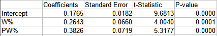
Looking at all of the W% inputs in this case (r^2 = .356) suggests that even though EW% was a more accurate predictor alone than PW%, it might be the variable to drop:

So with just W% and PW%, the r^2 is .354:
These results are not as clean as the year-over-year study; the sample size is smaller, and the results from using half the data to predict the other half and using both halves are inconsistent. The only conclusion that I feel comfortable drawing is that it’s unlikely that there is some kind of magic information encoded in a team’s actual W% in one set of games that predicts how it will do in another set of games, even within the same season.