
Pythagorean W% v. Next Year W%

2022 marks the fortieth anniversary of the first national publication of the Bill James Baseball Abstract, which one could posit was the beginning of a roughly thirty year process that took sabermetric analysis from something that had previously been the domain of a small group of pioneers (e.g. George Lindsey, Earnshaw Cook, Pete Palmer, Dick Cramer, Steve Mann) to an accepted part of the public’s collective conventional wisdom of baseball.
It is that phrase, “conventional wisdom”, that I was thinking about recently. Sabermetrics is now old enough as a field that there are things that James or Palmer may have originally studied a very long time ago, and there is a danger that findings could become venerated and not continually re-verified to still apply, or to stand up to more detailed data that is now available. So I started thinking about whether there were any propositions that I held in my head as some kind of conventional wisdom for which I could not point to a recent study that reaffirmed why I believed them to be true.
One that came to mind was the notion that expected win-loss records, based on runs/runs allowed ala Pythagorean, are more predictive of future win-loss records than actual win-loss records are. This is not a particularly important underpinning of sabermetrics, but it is certainly something that I believe to be true, and I know that I have seen studies that suggested it to be true, but I couldn’t cite any of them off the top of my head (despite being fairly certain that I had personally done some quick and dirty “studies” that confirmed that finding in some manner).
So I decided it might be worthwhile to do a very simple “study” to re-examine this issue. First, I should acknowledge that there are multiple ways in which the basic hypothesis could be defined, and I am only examining one of them. Namely, the claim could be that expected W%s are more predictive within a season, or that they are more predictive across seasons. A subset of this could be to question whether they are temporally oriented (i.e. first-half Pythagorean record is more predictive of second half actual win-loss record), or whether the finding would hold if say games were randomly selected into two buckets across all 162 games.
Here, I am only looking at the very straightforward question of how predictive expected W%s are of the following season’s W%, assuming a linear relationship between prior and future W%. The basics of my study are as follows:
* I considered all major league team-seasons from 1998 to 2018 as year one, and ran regressions using data from those seasons to predict each team’s record in year two (covering 1999 to 2019). I chose this time period as it covered a fairly robust 21 seasons, and also avoids any shortened seasons (which would pop up if the period extended back to 1995 or forward to 2020) and any seasons in which a team did not have a prior season to compare to (which would happen if 1997 was included as year one due to the 1998 expansion that added Arizona and Tampa Bay).
* I defined EW% as a team’s expected W% based on runs and runs allowed, using Pythagenpat with z = .29
* I defined PW% as a team’s predicted W% based on runs created and runs created allowed, again using Pythagenpat with the same exponent. I took a bit of a shortcut here, which was to use a simple linear formula for runs created (essentially Paul Johnson’s Estimated Runs Produced) and to just use the standard defensive statistical categories which don’t include the needed inputs at bats or total bases. Of course, these can be reasonably estimated from the standard categories, but it does introduce more potential for error when applying these formulas. The basic skeleton of the runs created formula I used, when all the data is available (as is the case for team offense) is:
TB + .8H + W - .3AB
A scalar multiplier is then applied to estimate runs scored; I determined this separately for each season (not split out by league) so that at the end league total R = RA = RC = RCA so that EW% and PW% are centered perfectly at .500. Of course, not taking this step would still results in average estimated W%s close to .500 as the formulas are reasonable and reliable estimates of runs scored. For 2019, the needed value was .3259, which was the highest over the 21 season; the lowest was .3148 for 2013. The RMSE of the team runs scored estimates is 22.65, which benefits from cheating by forcing the estimated league total to match actual league runs scored for each season.
For the defense, I estimated total bases and at bats using one relationship for the entire period, then applied the appropriate multiplier at the season level. It is convenient to rewrite the skeleton as the equivalent:
TB + .5H + W -.3(AB – H)
as innings can be directly related to batting outs (AB – H) as 2.836*IP = AB – H. To estimate total bases, we have hits and home runs allowed, so we can solve (H – HR)*x + HR*4 = TB for x to get 1.273 average total bases per non-HR hit, and now write the skeleton as:
1.273(H – HR) + 4HR + .5H + W -.3(2.836IP) = 1.773H + 2.727HR + W - .8508IP
For 2019, the needed multiplier is .3261, and the RMSE for the period is 25.60 – not as accurate as the offensive version, but good enough for the purpose of this study.
Now that we have defined EW% and PW%, the obvious step is to run regressions relating each of the three prior season W%s (which I will render in formulas without a prefix) to estimate the following season’s W% (which I will call next_W%). First, though, it is worthwhile to establish the error we would see in predicting the following season’s W% if we did not avail ourselves of any data from the prior season. Obviously, the most accurate estimate would be to assume that all teams would be .500, and thus the RMSE will equal the standard deviation of team wins for 1999 – 2019, since those are the “following” seasons in our scope. (Actually, the RMSEs I’m presenting are based on the RMSE for W% estimate multiplied by 162, but since almost all teams played 162 games it is of little consequence). The RMSE using .500 for all teams is 11.79.
If we use W% alone to estimate next_W%, the resulting equation is:
next_W% = .54541*W% + .22729
This produces a RMSE of 9.93 and a r^2 of .291. You will note that this is still a substantial error, although noticeable better than 11.79 from not having any knowledge of prior season performance. There are 630 teams included in the study; the absolute difference of next_W% and estimated next_W% is less than the absolute difference between next W% and .500 for 396 of them. In other words, considering the prior year’s W% enabled us to improve our prediction of the following year’s W% for 62.9% of teams. Along with the RMSE and r^2, we don’t see massively improved prediction - there is obviously a lot that goes into future season’s performance that isn’t evident from the prior season’s W%.
Can we capture some of this by considering EW% or PW%? In doing so, we will eliminate “sequencing luck” in terms of runs leading to wins in both cases, and in terms of discrete outcomes leading to runs in the latter case. Conventional sabermetric wisdom suggests that this should help, although we should also recognize that there are so many more determinants of the following season’s W% that aren’t considered that any improvements should be limited.
While I shouldn’t take a position in the search of objective knowledge about baseball, I am happy to report that the conventional wisdom holds - using EW% does improve the results slightly:
next_W% = .57847*EW% + .21057
This produces a RMSE of 9.84, r^2 of .304, and a better estimate for 401 teams (63.7%).
Using PW% improves things a bit more, suggesting that there maybe merit in discounting the predictive value of event sequencing (although since as alluded to earlier, there are myriad other factors that cause a team’s W% to change from season to season, it’s best not to get carried away with conclusions, and also note that the improvement is incremental):
next_W% = .65983*PW% + .17001
RMSE = 9.72, r^2 = .320, although it is better for only 388 teams (61.6%).
The natural next step is to take all three prior year W%s into account:
next_W% = .15755*W% + .01003*EW% + .48626*PW% + .17306
RMSE = 9.68, r^2 = .325, better for 388 teams (61.6%). While it’s discouraging that the three error metrics I’ve chosen (which certainly are not the only choices, but some of the most common) don’t all move together, in general this appears to be an improvement – except the coefficient for EW% is essentially zero, and its p-value is 0.94. For this particular dataset, it’s not adding any value beyond what we are getting from W% and PW%. So the best course of action is to eliminate it, and just run the regression using W% and PW% as independent variables:
next_W% = .16193*W% + .49228*PW% + .17287
RMSE = 9.68, r^2 = .325, better for 388 teams (61.6%). It should be unsurprising that the accuracy is the same since the formula is basically the same as EW% was not doing much.
No new ground has been covered here, but at least we do see some confirmation of the conventional sabermetric wisdom. To the extent that PW% is a better predictor of the following season’s W% than EW%, this has already been incorporated into widely disseminated statistics. Baseball Prospectus’ third-order W% are their version of what I call PW% adjusted for strength of schedule. Fangraphs’ Base Runs rooted win estimate are also what I would call PW%, using a superior run estimator to the linear one I’ve used here for the ease of looking at 21 seasons of data.
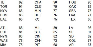
What fun would it be to run all these regressions and not close with the resulting estimates for 2022 (using W% and PW% as the independent variables)?
Related stuff...https://books.google.com/books?id=hR8sDAAAQBAJ&pg=PT95&lpg=PT95&dq=Bill+james+plexiglass+principle&source=bl&ots=IpKf-c_SD8&sig=ACfU3U3SscjWhXG5ZiWMfaTNlLV30HgmJQ&hl=en&sa=X&ved=2ahUKEwjay7LU47T2AhV6mWoFHSu1D5gQ6AF6BAgDEAE#v=onepage&q=Bill%20james%20plexiglass%20principle&f=false
Good stuff Patriot. And I agree, a good idea to have a reference study.
Tiny note for those who don't see this as obvious. This:
next_W% = .65983*PW% + .17001
Which if we round is this:
next_W% = .66*PW% + .17
Can be rewritten as this:
next_W% = .66*(PW% - .500) + .500
In other words, we regress by 34%.
That .66 therefore can be rewritten as this:
162 / (162 + 83 )
That 83 is the "ballast". And this means you can have a generalized equation for any number of games. If you had for example only a 60 game season, then the predictor would be this:
next_W% = .42*(PW% - .500) + .500